概述

2018年3月23日

数学笔记：概率、期望

期望（Expectation）的定义如果X是在概率空间[latex] (\Omega, …

by KSkun

2018年3月23日

概述

拉格朗日插值法常用于通过点值获得满足这些点值的多项式，是一种由点值到多项式的转换方式。下面介绍其原理及应用。

过程

对于某个k次多项式函数，已知给定k+1个取值点，分别为[latex] (x_0, y_0), \ldots, (x_k, y_k) [/latex]。
假设这些点的x值都不同，那么对于每个点我们写出它的拉格朗日基本多项式（插值基函数），为
[latex display=”true”] \ell_j(x) = \prod_{i=0, i \neq j}^k \frac{x-x_i}{x_j-x_i} [/latex]
再利用这些多项式构成拉格朗日插值多项式，为
[latex display=”true”] L(x) = \sum_{j=0}^k y_j \ell_j(x) [/latex]
我们容易观察到，拉格朗日基本多项式的特点是只有当x值为[latex]x_j[/latex]时取值为1，其他点值的x值的取值都为0。

例子

假如我们需要求出某个二次多项式函数f，我们知道了三个点值(1, 1)、(2, 4)和(3, 9)，下面构造它们的拉格朗日基本多项式
[latex display=”true”] \begin{aligned} \ell_0(x) &= \frac{(x-2)(x-3)}{2} \\ \ell_1(x) &= -(x-1)(x-3) \\ \ell_2(x) &= \frac{(x-1)(x-2)}{2} \end{aligned} [/latex]
加起来，得到了
[latex display=”true”] f(x) = x^2 [/latex]

算法

点值求多项式：[latex]O(n^2)[/latex]
多项式求值：[latex]O(n^2)[/latex]

by KSkun

[51Nod1716]多项式？题解

题目地址：51Nod：多项式？问题 – 51Nod 题目描述现在有一个n次 …

题解, 算法, 其他

by KSkun

数学笔记：泰勒公式、泰勒级数、泰勒展开

别看这个标题上有三个名词，其实他们说的都是一个东西，就是下面的这个玩意：泰勒定理（Tay …

by KSkun

[NOI2001]反正切函数的应用题解

题目地址：POJ：1183 — 反正切函数的应用

题目描述

反正切函数可展开成无穷级数，有如下公式
[latex display=”true”]\arctan x = \sum_{n=0}^\infty \frac{(-1)^n x^{2n+1}}{2n+1} \ (0 \leq x \leq 1) \ (1)[/latex]
使用反正切函数计算[latex]\pi[/latex]是一种常用的方法。例如，最简单的计算[latex]\pi[/latex]的方法：
[latex display=”true”]\begin{aligned} \pi & = 4 \arctan 1 \\ & = 4(1 – \frac{1}{3} + \frac{1}{5} – \frac{1}{7} + \frac{1}{9} – \frac{1}{11} + \cdots) \ (2) \end{aligned}[/latex]
然而，这种方法的效率很低，但我们可以根据角度和的正切函数公式：
[latex display=”true”]\tan(\alpha + \beta) = \frac{\tan \alpha + \tan \beta}{1 – \tan \alpha \tan \beta} \ (3)[/latex]
通过简单的变换得到：
[latex display=”true”]\arctan p + \arctan q = \arctan(\frac{p+q}{1-pq}) \ (4)[/latex]
利用这个公式，令[latex]p=\frac{1}{2}, q=\frac{1}{3}[/latex]，则[latex]\frac{p+q}{1-pq} = 1[/latex]，有
[latex display=”true”]\arctan \frac{1}{2} + \arctan \frac{1}{3} = \arctan(\frac{\frac{1}{2} + \frac{1}{3}}{1 – \frac{1}{2} \times \frac{1}{3}}) = \arctan 1[/latex]
使用[latex]\frac{1}{2}[/latex]和[latex]\frac{1}{3}[/latex]的反正切来计算[latex]\arctan 1[/latex]，速度就快多了。
我们将公式(4)写成如下形式
[latex display=”true”]\arctan \frac{1}{a} = \arctan \frac{1}{b} + \arctan \frac{1}{c}[/latex]
其中a、b和c均为正整数。
我们的问题是：对于每一个给定的a（1≤a≤60000），求b+c的值。我们保证对于任意的a都存在整数解。如果有多个解，要求你给出b+c最小的解。

输入输出格式

输入格式：
输入文件中只有一个正整数a，其中1≤a≤60000。

输出格式：
输出文件中只有一个整数，为b+c的值。

输入输出样例

输入样例#1：

输出样例#1：

题解

本题为推式子题，内容不会超过高中知识范畴，请各位放心食用。
首先我们将给定式进行公式(4)的变换，得到的式子如下
[latex display=”true”]\arctan \frac{1}{a} = \arctan(\frac{\frac{1}{b} + \frac{1}{c}}{1 – \frac{1}{bc}})[/latex]
进而因为反正切函数的性质，可以直接得到
[latex display=”true”]\frac{1}{a} = \frac{\frac{1}{b} + \frac{1}{c}}{1 – \frac{1}{bc}}[/latex]
进行化简后可以得到
[latex display=”true”]a = \frac{bc-1}{b+c}[/latex]
b和c都在式子里不好处理，我们考虑用[latex]S=b+c[/latex]把其中一个消掉，然后把S表示成另一个的函数，函数写出来如下
[latex display=”true”]S(c) = c + a + \frac{a^2+1}{c-a}[/latex]
现在我们对这个函数在正整数范围内求最小值，如果不考虑整数，我们可以利用均值不等式知道最小值应该在[latex]c = a + \sqrt{a^2 + 1}[/latex]处取到，但是此时函数值可能不是一个整数，不满足b、c都是正整数的条件。因此我们可以考虑在这个值附近枚举c。因为这是一个双曲线，最小整点在临界点两边取得都有可能，那我们就在两边枚举就好了。
其实你还可以接着分析，因为c越靠近a，函数值增长得越快，越远离a，函数值增长的越慢，一般来说应该在向左枚举的过程中最先找到整点吧。但是这个还没办法证明。

代码

// Code by KSkun, 2018/3
#include <cstdio>
#include <cmath>

typedef long long LL;

LL a;

inline LL cals(LL c) {
    return c + a + (a * a + 1) / (c - a);
}

int main() {
    scanf("%lld", &a);
    LL c = a + sqrt(a * a + 1), c1 = c, c2 = c;
    for(;; c1--, c2++) {
        if((c1 - a) && (a * a + 1) % (c1 - a) == 0) {
            printf("%lld", cals(c1));
            break;
        }
        if((c2 - a) && (a * a + 1) % (c2 - a) == 0) {
            printf("%lld", cals(c2));
            break;
        }
    }
    return 0;
}

题解, 算法, NOI系列

by KSkun

拉格朗日乘数法及其应用

概述拉格朗日乘数法是数学中一种求带限制时多元函数的极值的常用方法。下面我们介绍拉格朗日乘 …

by KSkun

4 Comments

2018年3月21日

[NOI2012]骑行川藏题解

题目地址：洛谷：【P2179】[NOI2012]骑行川藏 – 洛谷、BZOJ： …

题解, 算法, NOI系列

by KSkun

2018年3月21日

数学笔记：极限、导数、积分

极限（Limit）

概念

c，L皆为实数，[latex]f: (- \infty, c – \delta) \cup (c + \delta, + \infty) \rightarrow \mathbb{R}[/latex]，当[latex]x \rightarrow c[/latex]时，[latex]f(x) \rightarrow L[/latex]当且仅当：任一个[latex]\epsilon > 0[/latex]，必存在一个[latex]\delta > 0[/latex]，使得若[latex]0 < |x – c| < \delta[/latex]，则[latex]|f(x) – L| < \epsilon[/latex]。

通俗理解

当x趋向于某值L时，f(x)的值趋向于某值A。

表达

符号表达：[latex]\lim_{x \rightarrow x_0} f(x) = A[/latex]
特殊记号：
[latex]x \rightarrow x_0^+[/latex]：x从右侧趋向于[latex]x_0[/latex]，x恒大于[latex]x_0[/latex]。
[latex]x \rightarrow x_0^-[/latex]：x从左侧趋向于[latex]x_0[/latex]，x恒小于[latex]x_0[/latex]。

四则运算

[latex display=”true”]\begin{aligned} \lim_{x \rightarrow x_0} (f(x) + g(x)) &= \lim_{x \rightarrow x_0} f(x) + \lim_{x \rightarrow x_0} g(x) \\ \lim_{x \rightarrow x_0} (f(x) – g(x)) &= \lim_{x \rightarrow x_0} f(x) – \lim_{x \rightarrow x_0} g(x) \\ \lim_{x \rightarrow x_0} (f(x) \cdot g(x)) &= \lim_{x \rightarrow x_0} f(x) \cdot \lim_{x \rightarrow x_0} g(x) \\ \lim_{x \rightarrow x_0} \frac{f(x)}{g(x)} &= \frac{\lim_{x \rightarrow x_0} f(x)}{\lim_{x \rightarrow x_0} g(x)} \end{aligned}[/latex]

夹逼定理（Squeeze theorem）

设I为包含某点a的区间，f，g，h为定义在I上的函数。若对于所有属于I而不等于a的x，有：[latex]g(x) \leq f(x) \leq h(x)[/latex]且[latex]\lim_{x \rightarrow a} g(x) = \lim_{x \rightarrow a} h(x) = L[/latex]，则[latex]\lim_{x \rightarrow a} f(x) = L[/latex]。
其中，g(x)和h(x)分别称为f(x)的下界和上界。

连续函数（Continuous function）

对于定义域I中任意[latex]x_0[/latex]，有[latex]\lim_{x \rightarrow x_0} = f(x_0)[/latex]，则称f(x)是一个连续函数。
注：本定义不严谨，只用于说明极限可用于定义连续函数。严谨定义参见连续函数 – 维基百科，自由的百科全书。
函数的连续性与（处处）连续的函数并不相同。函数可以在一段区间内连续，也就是说，连续性是一个局部性质。
复合的连续函数也是连续的。初等函数是连续的。

常用的结论

[latex display=”true”]\begin{aligned} &\lim_{x \rightarrow + \infty} (1 + \frac{1}{n})^n = \lim_{x \rightarrow – \infty} (1 + \frac{1}{n})^n = e \\ &\lim_{x \rightarrow 0} \frac{\sin x}{x} = \lim_{x \rightarrow 0} \frac{\tan x}{x} = 1 \\ &\lim_{x \rightarrow + \infty} \sqrt[n]{n} = 1 \\ &\lim_{x \rightarrow 0} \frac{\arctan x}{x} = \lim_{x \rightarrow 0} \frac{e^x – 1}{x} = 1 \end{aligned}[/latex]

等价无穷小（大）量

设f在区间I上有定义，[latex]x_0[/latex]在I中，若[latex]\lim_{x \rightarrow x_0} f(x) = 0[/latex]，则称f为当[latex]x \rightarrow x_0[/latex]时的无穷小量。
设当[latex]x \rightarrow x_0[/latex]时，f与g均为无穷小量，若[latex]\lim_{x \rightarrow x_0} \frac{f(x)}{g(x)} = 1[/latex]，则称f与g是当[latex]x \rightarrow x_0[/latex]时的等价无穷小量，记作[latex]f(x) \sim g(x) \ (x \rightarrow x_0)[/latex]。
类似地，等价无穷大量也可以如此定义。求极限时，可以利用它的性质进行代换。

高（低）阶无穷小量

对于两个无穷小量[latex]\alpha[/latex]和[latex]\beta[/latex]，如果[latex]\lim \frac{\alpha}{\beta} = 0[/latex]，称[latex]\alpha[/latex]为比[latex]\beta[/latex]高阶的无穷小量，简称高阶无穷小量。类似地，[latex]\beta[/latex]是[latex]\alpha[/latex]的低阶无穷小。记作[latex]\alpha = o(\beta)[/latex]。
通俗理解，在某一趋近过程中，[latex]\alpha \rightarrow 0[/latex]比[latex]\beta \rightarrow 0[/latex]快一些。

导数（Derivative）

概念

当函数f的自变量在一点[latex]x_0[/latex]上产生一个增量h时，函数输出值的增量与自变量增量h的比值在h趋于0时的极限如果存在，即为f在[latex]x_0[/latex]chu处的导数，记作[latex]f'(x_0)[/latex]。
对于可导的函数f，[latex]x \mapsto f'(x)[/latex]也是一个函数，称为f的导函数。
已知函数求导函数的过程为求导，已知导数求原函数的过程为不定积分。
对于连续函数图像，其一点处的导数即为图像在该点处切线的斜率。

运算与复合函数规律

[latex display=”true”]\begin{aligned} (f(x) + g(x))’ &= f'(x) + g'(x) \\ (f(x) – g(x))’ &= f'(x) – g'(x) \\ (f(x) \cdot g(x))’ &= f'(x) \cdot g(x) + g'(x) \cdot f(x) \\ (\frac{f(x)}{g(x)})’ &= \frac{f'(x) \cdot g(x) + g'(x) \cdot f(x)}{g^2(x)} \\ (f(g(x)))’ &= f'(g(x)) \cdot g'(x) \end{aligned}[/latex]

初等函数的求导

常函数：[latex]f(x) = c, f'(x) = 0[/latex]
多项式函数：[latex]f(x) = x^a \ (a \in \mathbb{Q}^*), f'(x) = ax^{a-1}[/latex]
三角函数：[latex]f(x) = \sin x, f'(x) = \cos x[/latex]；[latex]f(x) = \cos x, f'(x) = – \sin x[/latex]
指数函数：[latex]f(x) = a^x, f'(x) = a^n \ln a[/latex]；特例：[latex]f(x) = e^x, f'(x) = e^x[/latex]
对数函数：[latex]f(x) = \log_a x, f'(x) = \frac{1}{x \ln a}[/latex]；特例：[latex]f(x) = \ln x, f'(x) = \frac{1}{x}[/latex]

洛必达法则（L’Hospital’s rule）

[latex]x \rightarrow x_0, f(x), g(x) \rightarrow 0[/latex]，且[latex]x \rightarrow x_0, \frac{f'(x)}{g'(x)} = A[/latex]，则[latex]x \rightarrow x_0, \frac{f(x)}{g(x)} = \frac{f'(x)}{g'(x)} = A[/latex]。
注：严谨的表述见洛必达法则 – 维基百科，自由的百科全书。

偏导数（Partial derivative）

多元函数的偏导数是它关于其中一个变量的导数，而保持其他变量恒定（当成常数处理）。
函数f关于变量x的偏导数记为[latex]\frac{\partial f}{\partial x}[/latex]。

积分（Integral）

定积分

定积分的定义有很多种，这里给出一个直观的描述。
对于一个给定的实值函数f(x)，f(x)在一个实数区间[a, b]上的定积分[latex]\int_a^b f(x)\rm{d}x[/latex]可以理解为在Oxy坐标平面上，曲线y=f(x)与x轴、直线x=a、直线x=b围成的有向面积。有向面积是指，x轴上方的面积为正，下方的面积为负。
注：定义参见积分 – 维基百科，自由的百科全书。

不定积分

f的不定积分（或称原函数）是任何满足其导函数是函数f的函数F。一个函数f的不定积分不是唯一的。
[latex display=”true”]\int f(x)\mathrm{d}x = F(x) + C[/latex]
其中[latex]f = F[/latex]是[latex]f = f[/latex]的不定积分。

微积分（第二）基本定理（牛顿-莱布尼茨公式）

[latex display=”true”]\int_a^b f(x)\mathrm{d}x = F(b) – F(a)[/latex]
其中，[latex]F'(x) = f(x)[/latex]。
图形化的直观理解见下图。

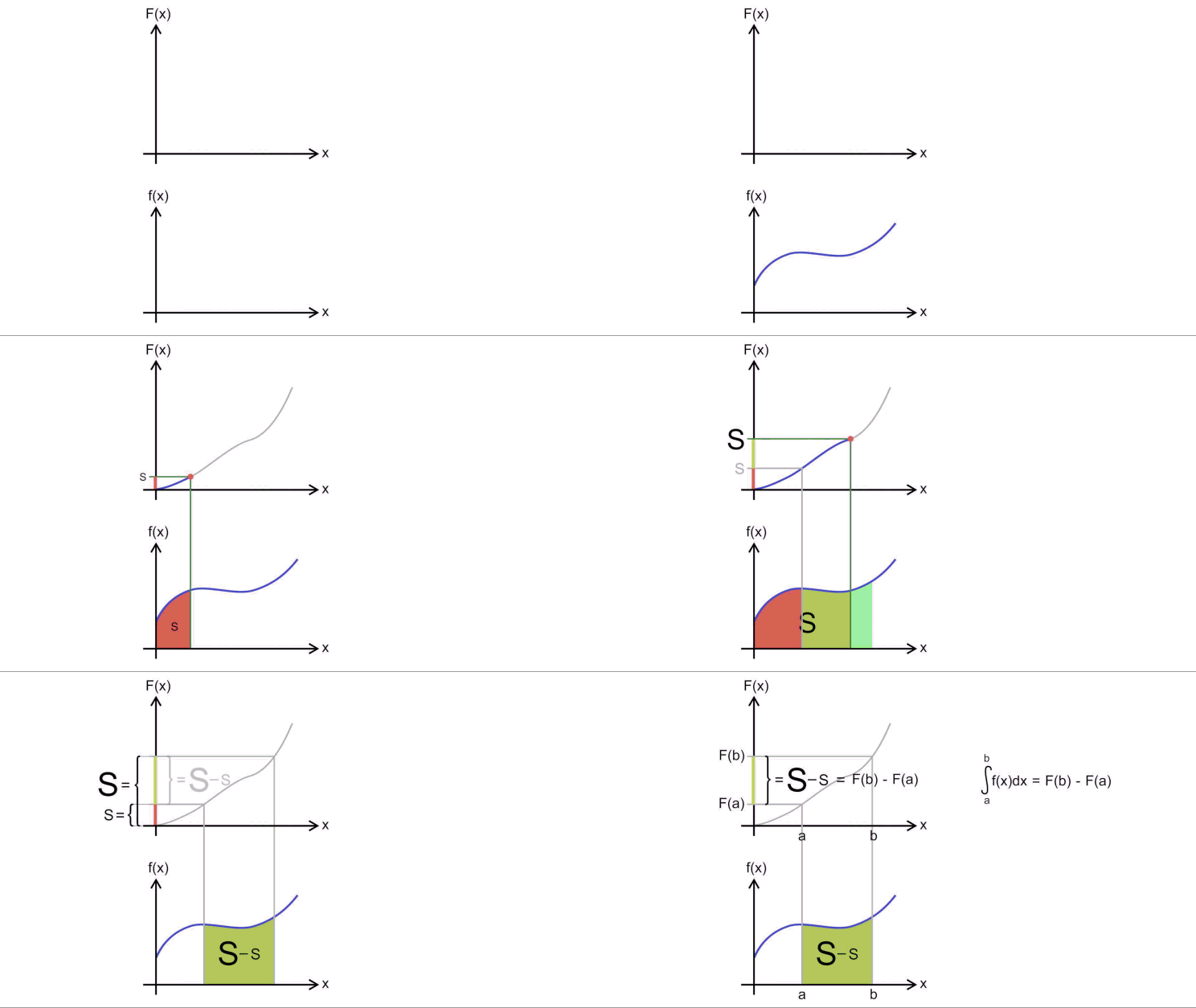
（图片来自维基百科：微积分基本定理 – 维基百科，自由的百科全书）

常用结论

[latex]\int x^k \mathrm{d}x = \frac{1}{k+1} x^{k+1} + C[/latex]
分部积分法：[latex]\int f(x)g'(x)\mathrm{d}x = \int f(x)\mathrm{d}g(x) = f(x)g(x) – \int g(x)f'(x)\mathrm{d}x[/latex]
[latex]\int e^x \mathrm{d}x = e^x + C[/latex]
[latex]\int \frac{1}{x} \mathrm{d}x = \ln |x| + C[/latex]

贝塔函数（Beta function，第一类欧拉积分）

[latex display=”true”] \mathrm{B}(x, y) = \int_0^1 t^{x-1}(1-t)^{y-1}\mathrm{d}t [/latex]
性质：

对称性：[latex]\mathrm{B}(x, y) = \mathrm{B}(y, x)[/latex]
与伽马函数之间的关系：[latex]\mathrm{B}(x, y) = \frac{\Gamma(x) \Gamma(y)}{\Gamma(x+y)}[/latex]
当x, y是正整数时，有[latex]\mathrm{B}(x, y) = \frac{(x-1)!(y-1)!}{(x+y-1)!}[/latex]

其他性质参见：Β函数 – 维基百科，自由的百科全书

伽马函数（Gamma function，第二类欧拉积分）

[latex display=”true”] \Gamma(z) = \int_0^\infty \frac{t^{z-1}}{e^t} \mathrm{d}t [/latex]
如果n为正整数，则
[latex display=”true”] \Gamma(n) = (n-1)! [/latex]
其他性质参见：Γ函数 – 维基百科，自由的百科全书

参考资料

by KSkun

2018年2月23日

[THUT2012]序列操作题解

题目地址：洛谷：【P4247】[清华集训]序列操作 – 洛谷、BZOJ：Pro …

题解, 算法, NOI系列

by KSkun